A DIY Dashboard with Grafana

Oct 30, 2017

13 minute read

DevOps

If your code creates some stats to monitor, Grafana and the Grada package may come in handy.

Recently I had some time to play with Grafana ( GitHub page, home page), an open-source data dashboard for monitoring all kinds of time series data.

While Grafana comes with many prebuilt data sources for well-known metrics collector services and time series databases, I immediately thought of something different: what if I could feed a time series from my own code into a Grafana dashboard?

Turned out that there is an easy way to do that, with the help of a generic backend datasource named “SimpleJson”. This datasource first sends a JSON query to a given URL, in order to retrieve the available metrics from that server. After connecting a dashboard panel to a metric, Grafana can query the server periodically for metrics data.

To easily connect any Go code to a Grafana dashboard panel, I wrote the package grada (from GRAfana DAshboard) that collects simple time series data and makes this data available to a Grafana instance via an HTTP server running in the background.

(Note that at the time of this writing, grada is only a proof of concept, and is not intended for use in production environments.)

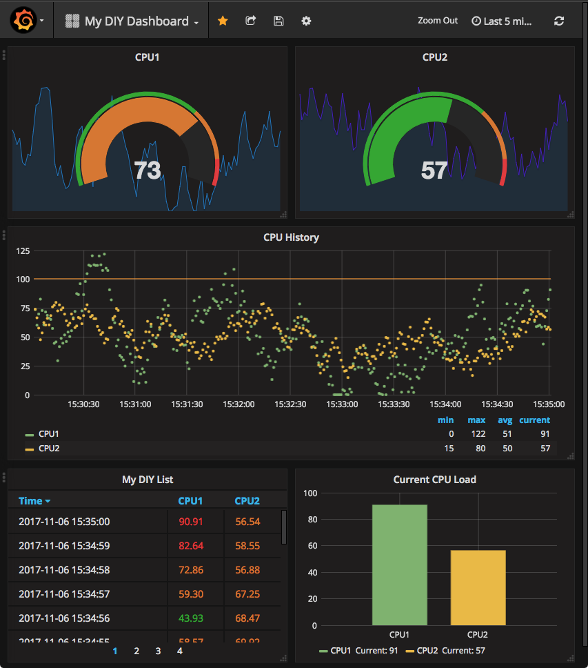
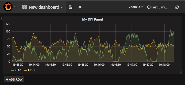
In this article, I will walk you through the steps of writing some sample code and setting up a local Grafana server, so that you can start creating dashboards like this one:

The DIY Dashboard

Let’s start by writing the test code. The reason for doing this first is that when we set up Grafana, our server should already be up and running, so that we immediately can connect to our custom data source and see if everything works as intended.

Using grada for collecting time series data

The small piece of code that follows demonstrates how to create two custom metrics and two data feeds. The data is the current CPU load of two CPU cores, captured every second. I was not able to find a package that can read CPU load on at least the three major OSes (Linux, macOS, and Windows), and so I created a fake CPU load generator instead. The point is to see some nice graphs on the screen, and you can replace that data generator with some useful, real data source later.

So let’s start!

Imports and globals

package main

import (
	"log"
	"math"
	"math/rand"
	"time"

This is the grada package. (It has no dependencies other than stdlib.)

	"github.com/christophberger/grada"
)

The data generator

This function creates a stream of data that simulates a source of constantly, but not entirely randomly, changing values.

max suggests an upper limit, which, however, the algorithm might occasionally exceed. The lower limit is 0.

volatility controls the speed of change, loosely speaking.

responseTime specifies a simulated response time (in milliseconds) of our imaginary data stream.

func newFakeDataFunc(max int, volatility float64, responseTime int) func() float64 {
	value := rand.Float64()
	return func() float64 {
		time.Sleep(time.Duration(responseTime) * time.Millisecond) // simulate response time
		rnd := 2 * (rand.Float64() - 0.5)
		change := volatility * rnd
		change += (0.5 - value) * 0.1
		value += change
		return math.Max(0, value*float64(max))
	}
}

Create and run two test metrics

In main(), we do just a few steps:

Create two Metric objects. A Metric is basically a ring buffer large enough to store timestamped data for the time range that Grafana asks for. Each Metric object has a name, in order to identify itself. Later, you will see these names appearing in Grafana when connecting a panel to a metric.
Create two data sources. Each data source delivers a number between 0 and (about) 100, at a rate of one number per second.
Define a function that polls a data source and adds the result to a metric.
Run that function in two goroutines, one goroutine per metric.

This handful of steps is enough to get our time series data flowing.

Here are the details:

func main() {

Here we set up the dashboard. This automatically starts the HTTP server in the background that will answer the requests from the Grafana dashboard.

	dash := grada.GetDashboard()

Then, we create two Metrics with target names “CPU1” and “CPU2”, respectively.

We want to save enough data for a 5-minute time range, at an incoming data rate of one value per second.

	CPU1metric, err := dash.CreateMetric("CPU1", 5*time.Minute, time.Second)
	if err != nil {
		log.Fatalln(err)
	}

The same as above, but this time, we specify the buffer size directly.
5 mins = 300 seconds = 300 data points needed

	CPU2metric, err := dash.CreateMetricWithBufSize("CPU2", 300)
	if err != nil {
		log.Fatalln(err)
	}

Now we need some simulated data streams. newFakeDataFunc() delivers exactly this.

	CPU1stats := newFakeDataFunc(100, 0.2, 1000)
	CPU2stats := newFakeDataFunc(100, 0.1, 1000)

In order to poll two data streams at the same time, we need to spawn one goroutine per data stream. This function will become the body of those goroutines.
To keep things simple, this code intentionally lacks any sort of goroutine cancellation mechanism. The function simply runs until the user hits Ctrl-C.
The loop rate is automatically limited by dataFunc() that returns only if a new value is available.

	trading := func(metric *grada.Metric, dataFunc func() float64) {
		for {
			metric.Add(dataFunc())
		}
	}

Let’s spawn the two goroutines now.

	go trading(CPU1metric, CPU1stats)
	go trading(CPU2metric, CPU2stats)

A quick and dirty way of waiting for Ctrl-C. An empty select{} always blocks.

Hit Ctrl-C to stop the app.


	select {}
}

Two caveats

There are two things to consider when using grada.

First, when creating a metric, choose the longest time range that the dashboard might request. For example, if you plan to monitor data from the last 24 hours at most, choose this timeframe, even if most of the time, you set the dashboard to monitor only the last half an hour or so.

The Metric type stores exactly the amount of data points that can occur for the given time range and the given data rate.

For example, if your code delivers new data every 5 seconds, and if the maximum time range to monitor is 5 minutes, only the most recent 60 data points are stored (5min * 60s/min / 5s).

Second, all data points are stored in memory. Each data point is a struct containing a float64 and a time.Time value. This struct consumes 32 bytes. There is no persistant storage behind a Metric object; so if you plan to monitor large time ranges and/or high-frequency data sources, verify if the required buffer still fits into main memory.

How to get and run the code

Step 1: go get the code. Note the -d flag that prevents auto-installing the binary into $GOPATH/bin.

go get -d github.com/appliedgo/diydashboard

Step 2: cd to the source code directory.

cd $GOPATH/src/github.com/appliedgo/diydashboard

Step 3. Run the binary.

go run diydashboard.go

Now the server is up and running, and the data sources start generating data. In the next step, we install Grafana.

Install and run Grafana

Grafana comes with OS-specific installation packages; feel free to pick the one that is for your OS and follow the installation documentation.

I will go a different way here and install Grafana as a Docker container. This is really easy and also almost the same on any platform that supports Docker. (When using macOS or Windows, keep in mind that Docker runs inside a Linux VM on these two platforms, but this should be no problem here. I run Docker on a Mac and it is almost the same as on Linux.)

The only downside is that the container needs to access a URL on the host machine, and there seems to be no universal solution for all OSes. (On a Mac, there is a dead easy solution, but on other OSes, your mileage may vary.)

So if you have Docker installed (or if you decide right now to install Docker), you may follow the steps I did. And here we go:

Step 1: Download and run the Grafana Docker image

At a shell prompt, run this command:

	docker run -d \
	-p 3000:3000 \
	--name grafana \
	--mount src=grafana-storage,dst=/var/lib/grafana \
	-e "GF_INSTALL_PLUGINS=grafana-simple-json-datasource" \
	grafana/grafana

Now that’s quite a mouthful of a command. Let’s take it apart and look what it does in detail:

Run a container in the background (-d).
Expose port 3000 to port 3000 on the host machine. (-p 3000:3000)
Name the container “grafana” (--name grafana)
Create and mount a Docker volume for persistent storage (--mount...)
Tell Grafana to install the SimpleJson datasource plugin (-e "GF_INSTALL_PLUGINS=..."). Grafana recognizes this environment variable, and downloads and installs the plugins listed there.
Run the container from the image grafana/grafana. Download the image (and all the required layers) from DockerHub/DockerStore, if required.

Whew! A simple docker run can actually do quite a lot behind the scenes. Now the container should be up and running. Test this by running

docker container ls

and you should see something like

CONTAINER ID        IMAGE               COMMAND             CREATED             STATUS              PORTS               NAMES
4bdb2ae2ef6c        grafana/grafana     "/run.sh"           39 seconds ago      Up 6 seconds                            grafana

If everything is ok so far, we can head over to step 2.

Step 2: There is no step 2.

Ok then… let’s move on to configuring Grafana.

Configuring a Grafana dashboard

Now it gets quite screenshot-ey! (Is this a word? Can I claim creatorship if no one subjects?) But as the saying goes, a picture is worth a thousand words, so here is the first one:

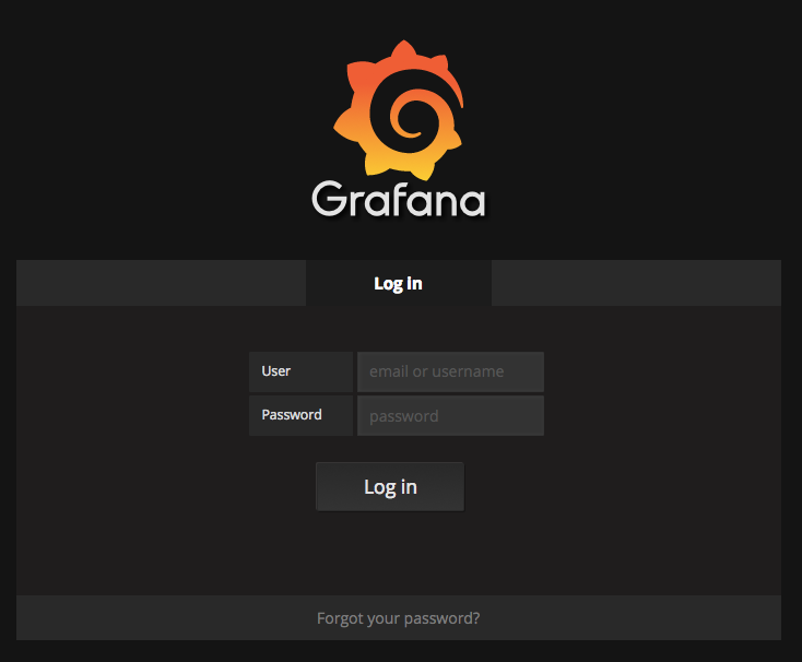
The default credentials are admin/admin. (You can of course change these after login.)

After successful login, we arrive at the Home Dashboard.

Home Dashboard

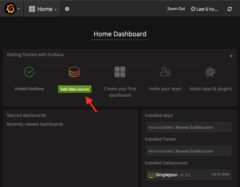
Create the data source

The first thing to set up is our custom data source. For this, click on “Add Data Source”.

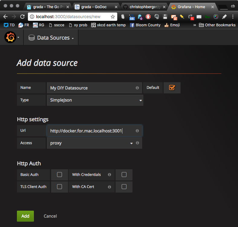
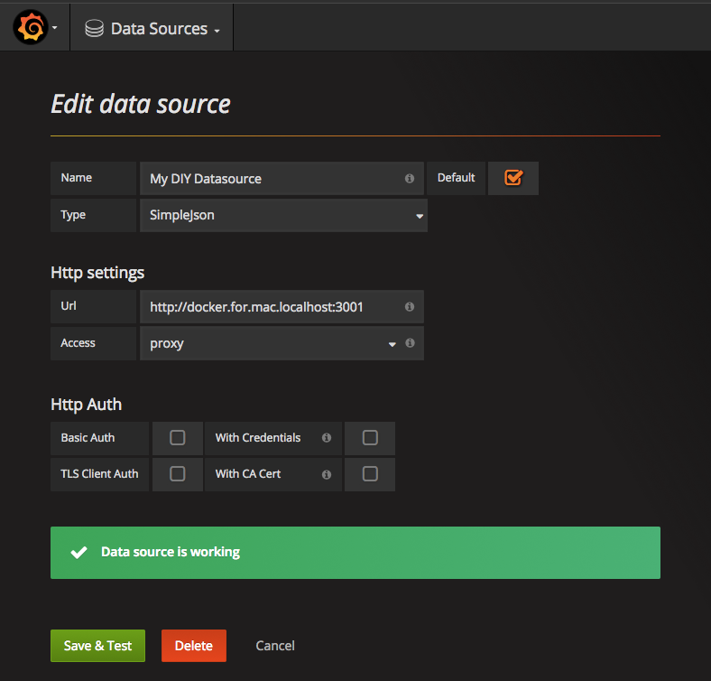
On the screen that opens, fill in the following fields:

Name: Choose a name you like.
Default: Ensure to check this box, so that new panels select this data source by default.
Type: Select “Simplejson”.
Url: This is where our Go code is listening. If you use Docker for Mac, set this to “http://docker.for.mac.localhost:3001”.
The Docker VM on macOS provides the “magic” URL “http://docker.for.mac.localhost” to access a Web server on the host machine, which I am using here. (Docker’s internal DNS resolves the domain name “docker.for.mac.localhost” to the host’s IP address, this is where the “magic” happens.)
On Linux or Windows you need to determine the host’s IP address as seen from within the container, and then use an URL like http://123.456.789.012:3001 to connect to the Go app.

The rest of the settings can be left as-is.

Add Datasource

Click Add to add this data source. Provided that the Go app is still running and the container network can access the host, the page should now look like this:

Datasource added

If everything looks fine, click the menu on the top left and select “Dashboards” to return to the Home Dashboard.

A tip if connecting to the host does not work

If you have trouble connecting from the Grafana container to the host machine, you can try two alternate options:

Option 1: Install Grafana locally without Docker, or
Option 2: Run the Go app within a Docker container, and connect the two containers via an internal network.

The second option takes only a few extra steps:

Step 1: Build and run a diydashboard container

Using the Dockerfile in $GOPATH/src/github.com/appliedgo/diydashboard, create a Docker container that contains nothing else but our Go app. The Dockerfile is a two-stage file.

FROM golang:latest AS buildStage
WORKDIR /go/src/diydashboard
COPY . .
RUN CGO_ENABLED=0 go get github.com/christophberger/grada
RUN CGO_ENABLED=0 go build

FROM scratch
WORKDIR /app
COPY --from=buildStage /go/src/diydashboard/diydashboard .
EXPOSE 3001
ENTRYPOINT ["/app/diydashboard"]

The first stage compiles the Go code into a binary. The second stage creates a container from the empty “scratch” image that contains just the diydashboard binary.

Run this Dockerfile in the shell, and start the resulting container:

cd $GOPATH/src/github.com/appliedgo/diydashboard
docker build -t diydashboard .
docker run --name diydashboard --rm -d diydashboard

** Step 2: Connect the two containers

Now we need to connect the Grafana container and the diydashboard container to the same internal Docker network. For this, we create a new network named “diy”.

docker network create diy
docker network connect diy grafana
docker network connect diy diydashboard

At this point, the grafana container can find the diydashboard container through its name. Docker’s internal DNS server maps the container name to the container’s IP address on the internal network.

So when you now insert the URL http://diydashboard:3001 and click Add (or Save & Test), you should now get the “Data source is working” message.

Add a dashboard

Now we can go ahead and create a dashboard.

For this, click on “Create your first dashboard”. The screen will change to:

New Dashboard

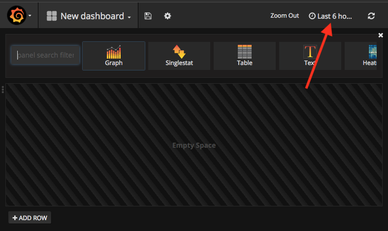
The first thing we do here is to change the time range that this dashboard requests from our data source. To do this, click the text in the upper right corner that says “Last 6 hours”.

On the dropdown that appears, click on “Last 5 minutes”.

To make the dashboard fetch new data regularly, click the “Refreshing every” dropdown box and select a suitable interval (say, 5s). Click “Apply” to save the settings.

Last 5 minutes

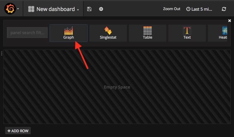
At the top of our still empty dashboard, there are a couple of panels to select from. Click on “Graph” to create a graph panel.

Add Panel

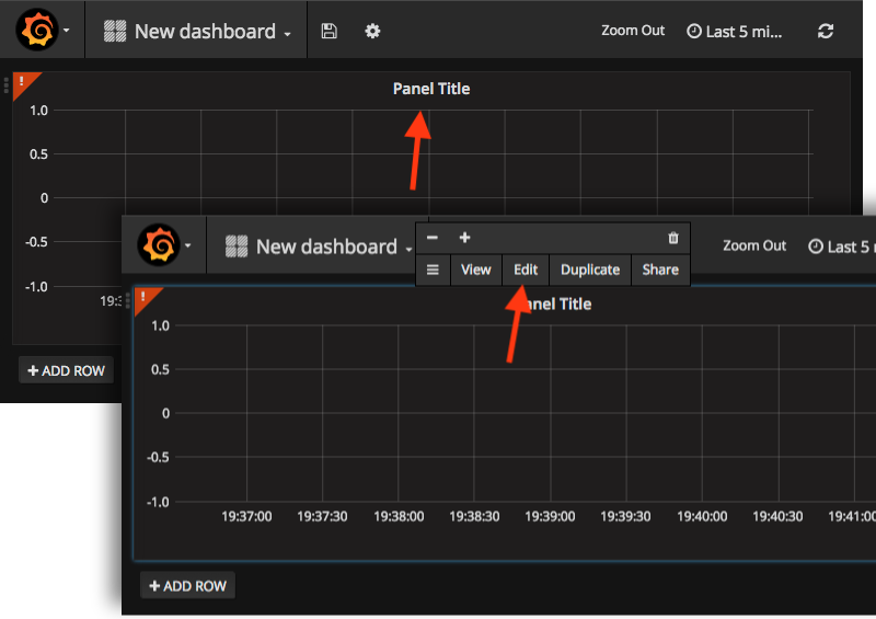
Now you see a new, empty panel. How do we bring it to life? The answer is not obvious. To configure the panel, click on its title. A popup dialog appears; click “Edit” to enter edit mode.j

Click Title and Edit

Ensure that the Metrics tab is active. This tab shows the data source that the panel reads from. If you have set the custom data source as default, you do not have to change the data source setting. Otherwise click on “default” and select the custom data source.

Below the data source, there are a couple of dropdown boxes. The first row says, “A”, “timeserie”, and “select metric”. This means that the panel expects to receive time series data. (The other option is “table” for receiving tabular data.)

Ensure that our Go app is still running, then click on “select metric”.

Select Metric

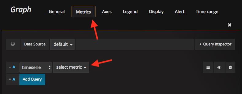
In the dropdown that opens, you should see the two data sources “CPU1” and “CPU2” that we created in the Go app. Grafana queries our app for all available metrics and presents them here.

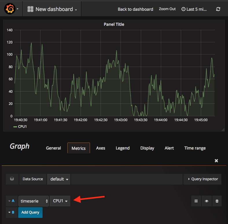
Select “CPU1”, and the graph area should immediately show some data, as far as the Go app has already generated it after starting.

CPU1 Selected

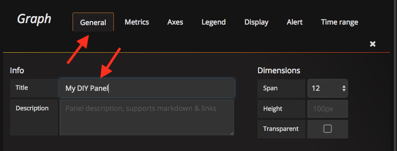
A dashboard can contain many panels, so you will want to give each panel a name. This also just needs a few clicks: Select the “General” tab, and then change the Title string to a really meaningful name like, “My DIY Panel”.

Change Title

If you want, you can have the panel show more than one metric. Our app generates two metrics, so let’s add “CPU2” to our panel.

CPU2 Selected

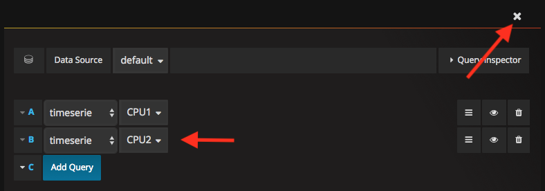
Click the close button in the top right corner to exit edit mode. If everything went fine, you should now see this:

Finished

Congrats! Your personal dashboard is up and running. You can now edit the panel again and play around with the look and feel, or you can add other panels like a single value (the “Singlestat” panel), a bar graph, or a plain list.

And, of course, you can go ahead and connect any time series data to the dashboard. How about network activity? Disk usage? The number of emails in your inbox? The temperature history of Death Valley? Or any other data you can think of (and find or write a Go library for).

Happy coding!