A Binary Search Tree
Search trees are everywhere: In databases, in file systems, in board game algorithms,… This post explores the probably most basic form of a tree: a binary search tree.
Table of contents
The Problem
Searching a value in a linear data container (list, array) with n elements can take up to n steps. Click on “Play” in the animation below and see how many steps it takes to find the value “3” when this value is in the last element of a list container.
Computer scientists say that this operation has an order of O(n). For very large values of n, this operation can become quite slow. Can we do better?
The Solution
If the data is organized in a tree structure, access can be much faster. Rather than 6 steps in the above example, the search takes only two steps:
The secret is that there is a sort order in this data structure. The search value is first compared against the value at the top of this structure. If the search value is smaller, the search continues with the next value to the left; else it continues with the next value to the right. Repeat until the value is found, or until there are no more values to the left or the right of the current value.
Binary Search Tree Basics
But wait, what is this “tree structure” seen in the animation above? This structure is called a binary search tree. It has the following properties:
- A tree consists of nodes that store unique values.
- Each node has zero, one, or two child nodes.
- One of the nodes is designated as the root node that is at the top of the tree structure. (This is the “entry point” where all operations start.)
- Each node has exactly one parent node, except for the root node, which has no parent.
- Each node's value is larger than the value of its left child but smaller than the value of its right child.
- Each subtree to the left of a node only contains values that are smaller than the node's value, and each subtree to the right of a node contains only larger values.
Some quick definitions that help keeping the following text shorter:
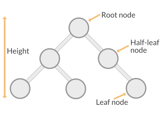
- A node with no children is called a leaf node.
- A node with one child is called a half leaf node.
- A node with two children is called an inner node.
- The longest path from the root node to a leaf node is called the tree's height.

In the best case, the height of a tree with n elements is log2(n+1) (where “log2” means the logarithm to base 2). All paths from the root node to a leaf node would have roughly the same length (plus/minus one). The tree is called a “balanced tree” in this case. Operations on this tree would have an order of *O(log(n)).
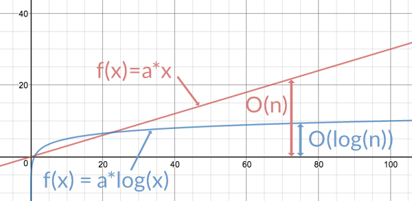
For large values of n, the logarithm of n is much smaller than n itself, which is why algorithms that need O(log(n)) time are much faster on average than algorithms that need O(n) time.
Take a calculator and find it out!
Let's say we have 1000 elements in our data store.
If the data store is a linear list, a search needs between 1 and 1000 steps to find a value. On average, this would be about 500 steps per search (if we assume the data is randomly distributed in this list).
If the data store is a balanced tree, a search needs at most log2(1001), or roughly 10 steps. What an improvement!
To visualize the difference, here is a diagram with a linear graph (in red) and a logarithmic graph (in blue). As the value on the x axis - the size of the data set - increases, the linear function keeps increasing with the same rate while the logarithmic function increases slower and slower the larger x gets.

Remember, O(log(n)) is only for the best case, where the tree is balanced, and no path to a leaf node is particularly longer than any other path.
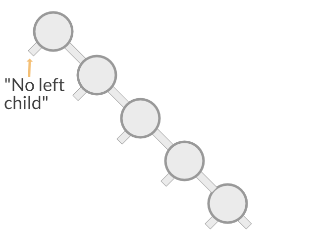
In this post, however, we look at a very simple binary search tree. Especially, we do not care to minimize the height of the search tree. So in the worst case, a tree with n elements can have a height of n, which means it is not better than a linear list. In fact, in this case, the tree is effectively a linear list:

So in the tree that we are going to implement, a search would take anywhere between O(log(n)) and O(n) time. In the next article, we'll see how to ensure that the tree is always balanced, so that a search always takes only O(log(n)) time.
Today's code: A simple binary search tree
Let's go through implementing a very simple search tree. It has three operations: Insert, Delete, and Find. We also add a Traverse function for traversing the tree in sort order.
Update: the balanced version of this code is now available in a generic version. See How I turned a binary search tree into a generic data structure with go2go · Applied Go
package main

import (
	"errors"
	"fmt"
	"log"
)
A Tree Node
Based on the above definition of a binary tree, a tree node consists of
- a value,
- a left subtree, and
- a right subtree.
By the way, this is a recursive data structure: Each subtree of a node is also a node containing subtrees.
In this minimal setup, the tree contains simple string data.
Node contains the search value, some data, a left child node, and a right child node.type Node struct {
Value string
Data string
Left *Node
Right *Node
}
Node Operations
Insert
To insert a value into a sorted tree, we need to find the correct place to add a new node with this value. Here is how:
- Start at the root node.
- Compare the new value with the current node's value.
- If it is the same, stop. We have that value already.
- If it is smaller, repeat 2. with the left child node. If there is no left child node, add a new one with the new value. Stop.
- IF it is greater, repeat 2. with the right child node, or create a new one if none exists. Stop.
Sounds quite easy, doesn't it? Just keep in mind we do not take care of keeping the tree balanced. Doing so adds a bit of complexity but for now we don't care about this.
The Insert method we define here works recursively. That is, it calls itself but with one of the child nodes as the new receiver. If you are unfamiliar with recursion, see the little example here or have a look at this factorial function.
Insert inserts new data into the tree, at the position determined by the search value.
Return values:trueif the data was successfully inserted,falseif the data value already exists in the tree.
func (n *Node) Insert(value, data string) error {

	if n == nil {
		return errors.New("Cannot insert a value into a nil tree")
	}

	switch {
	case value == n.Value:
		return nil
nil, insert a new left child node. Else call Insert on the left subtree. case value < n.Value:
if n.Left == nil {
n.Left = &Node{Value: value, Data: data}
return nil
}
return n.Left.Insert(value, data)
	case value > n.Value:
		if n.Right == nil {
			n.Right = &Node{Value: value, Data: data}
			return nil
		}
		return n.Right.Insert(value, data)
	}
	return nil
}
Find
Finding a value works as seen in the second animation of this article. (Hence, no animation here.) The Find method is also recursive.
It returns either the data of the found node and true, or "" and false if the node is not found.
Find searches for a string. It returns:- The data associated with the value and
true, or - "" and
falseif the search string is not found in the tree.
func (n *Node) Find(s string) (string, bool) {

	if n == nil {
		return "", false
	}

	switch {
	case s == n.Value:
		return n.Data, true
Find for the left child node, case s < n.Value:
return n.Left.Find(s)
Find for the right child node. default:
return n.Right.Find(s)
}
}
Delete
Deleting a value is a bit more complicated. Or rather, it is easy for two cases, and complicated for the third.
The easy cases:
Delete a leaf node.
This one is dead simple: Just set the parent's pointer to the node to nil.
Delete a half-leaf node.
Still easy: Replace the node by its child node. The tree's order remains intact.
The complicated case:
Delete an inner node.
This is the interesting part. The node to be deleted has two children, and we cannot assign both to the deleted node's parent node. Here is how this is solved. For simplicity, we assume that the node to be deleted is the right child of its parent node. The steps also apply if the node is the left child; you only need to swap “right” for “left”, and “large” for “small”.
- In the node's left subtree, find the node with the largest value. Let's call this node “Node B”.
- Replace the node's value with B's value.
- If B is a leaf node or a half-leaf node, delete it as described above for the leaf and half-leaf cases.
- If B is an inner node, recursively call the Delete method on this node.
The animation shows how the root node is deleted. This is a simple case where “Node B” is a half-leaf node and hence does not require a recursive delete.
To implement this, we first need two helper functions. The first one finds the maximum element in the subtree of the given node. The second one removes a node from its parent. To do so, it first determines if the node is the left child or the right child. Then it replaces the appropriate pointer with either nil (in the leaf case) or with the node's child node (in the half-leaf case).
findMax finds the maximum element in a (sub-)tree. Its value replaces the value of the
to-be-deleted node.
Return values: the node itself and its parent node.func (n *Node) findMax(parent *Node) (*Node, *Node) {
if n == nil {
return nil, parent
}
if n.Right == nil {
return n, parent
}
return n.Right.findMax(n)
}
replaceNode replaces the parent’s child pointer to n with a pointer to the replacement node.
parent must not be nil.func (n *Node) replaceNode(parent, replacement *Node) error {
if n == nil {
return errors.New("replaceNode() not allowed on a nil node")
}
if n == parent.Left {
parent.Left = replacement
return nil
}
parent.Right = replacement
return nil
}
Delete removes an element from the tree.
It is an error to try deleting an element that does not exist.
In order to remove an element properly, Delete needs to know the node's parent node.
parent must not be nil.func (n *Node) Delete(s string, parent *Node) error {
if n == nil {
return errors.New("Value to be deleted does not exist in the tree")
}
	switch {
	case s < n.Value:
		return n.Left.Delete(s, n)
	case s > n.Value:
		return n.Right.Delete(s, n)
	default:
		if n.Left == nil && n.Right == nil {
			n.replaceNode(parent, nil)
			return nil
		}
		if n.Left == nil {
			n.replaceNode(parent, n.Right)
			return nil
		}
		if n.Right == nil {
			n.replaceNode(parent, n.Left)
			return nil
		}
replacement, replParent := n.Left.findMax(n)
		n.Value = replacement.Value
		n.Data = replacement.Data
		return replacement.Delete(replacement.Value, replParent)
	}
}
The Tree
One of a binary tree's nodes is the root node - the “entry point” of the tree.
The Tree data type wraps the root node and applies some special treatment. Especially, it handles the cases where the tree is completely empty or consists of a single node.
The Tree data type also provides an additional function for traversing the whole tree.
Tree basically consists of a root node.type Tree struct {
Root *Node
}
Insert calls Node.Insert unless the root node is nilfunc (t *Tree) Insert(value, data string) error {
	if t.Root == nil {
		t.Root = &Node{Value: value, Data: data}
		return nil
	}
Node.Insert. return t.Root.Insert(value, data)
}
Find calls Node.Find unless the root node is nilfunc (t *Tree) Find(s string) (string, bool) {
if t.Root == nil {
return "", false
}
return t.Root.Find(s)
}
Delete has one special case: the empty tree. (And deleting from an empty tree is an error.)
In all other cases, it calls Node.Delete.func (t *Tree) Delete(s string) error {
if t.Root == nil {
return errors.New("Cannot delete from an empty tree")
}
Node.Delete. Passing a “fake” parent node here almost avoids
having to treat the root node as a special case, with one exception. fakeParent := &Node{Right: t.Root}
err := t.Root.Delete(s, fakeParent)
if err != nil {
return err
}
fakeParent. t.Root still points to the old node.
We rectify this by setting t.Root to nil. if fakeParent.Right == nil {
t.Root = nil
}
return nil
}
Traverse is a simple method that traverses the tree in left-to-right order
(which, by pure incidence ;-), is the same as traversing from smallest to
largest value) and calls a custom function on each node.func (t *Tree) Traverse(n *Node, f func(*Node)) {
if n == nil {
return
}
t.Traverse(n.Left, f)
f(n)
t.Traverse(n.Right, f)
}
A Couple Of Tree Operations
Our main function does a quick sort by filling a tree and reading it out again. Then it searches for a particular node. No fancy output to see here; this is just the proof that the whole code above works as it should.
mainfunc main() {
	values := []string{"d", "b", "c", "e", "a"}
	data := []string{"delta", "bravo", "charlie", "echo", "alpha"}
	tree := &Tree{}
	for i := 0; i < len(values); i++ {
		err := tree.Insert(values[i], data[i])
		if err != nil {
			log.Fatal("Error inserting value '", values[i], "': ", err)
		}
	}
	fmt.Print("Sorted values: | ")
	tree.Traverse(tree.Root, func(n *Node) { fmt.Print(n.Value, ": ", n.Data, " | ") })
	fmt.Println()
	s := "d"
	fmt.Print("Find node '", s, "': ")
	d, found := tree.Find(s)
	if !found {
		log.Fatal("Cannot find '" + s + "'")
	}
	fmt.Println("Found " + s + ": '" + d + "'")
	err := tree.Delete(s)
	if err != nil {
		log.Fatal("Error deleting "+s+": ", err)
	}
	fmt.Print("After deleting '" + s + "': ")
	tree.Traverse(tree.Root, func(n *Node) { fmt.Print(n.Value, ": ", n.Data, " | ") })
	fmt.Println()
Tree.Delete about why this is a special case.) fmt.Println("Single-node tree")
tree = &Tree{}
tree.Insert("a", "alpha")
fmt.Println("After insert:")
tree.Traverse(tree.Root, func(n *Node) { fmt.Print(n.Value, ": ", n.Data, " | ") })
fmt.Println()
tree.Delete("a")
fmt.Println("After delete:")
tree.Traverse(tree.Root, func(n *Node) { fmt.Print(n.Value, ": ", n.Data, " | ") })
fmt.Println()
}
The code is on GitHub. Use -d on go get to avoid installing the binary into $GOPATH/bin.
go get -d github.com/appliedgo/bintree
cd $GOPATH/src/github.com/appliedgo/bintree
go build
./bintree
Conclusion
Trees are immensely useful for searching and sorting operations. This article has covered the most basic form of a search tree, a binary tree. Other variations of trees exist (and are widely used), for example, trees where nodes can have more than two children, or trees that store data in leaf nodes only. None of these variations are inherently better; each has its particular use case(s).
You surely have noticed that most of the methods used here are written in a recursive manner. To keep your fingers exercised, rewrite those methods without using recursion.
Find out more about binary search trees on Wikipedia.
In the next article on binary trees, we will see how to keep the tree balanced, to achieve optimal search performance.
Until then!
Changelog
2016-08-07 Fixed:
\4. Each node's value is larger than the value of its left child but larger than the value of its right child.
\4. Each node's value is larger than the value of its left child but smaller than the value of its right child.
2016-08-07 Fixed: missing return in replaceNode.
2016-08-27 Fixed typo: “Base on”
2016-11-26: Fixed corner case of deleting the root note of a tree if the root node is the only node.

Imports and globals