Imagine you just finished writing some code to solve a particular problem. The input is an array of values, and your code calculates some result from this array. You benchmark the code and find that it is reasonably fast for your test data.

Later, you get your hands on some real big data set from your production systems. A hundred times larger than your test data. “Ok,” you tell yourself, “if I run the benchmark with this input, my code should take a hundred times as long as with my test data.”

To your surprise, the code takes a thousand times longer! What happened?

The problem of input size

Whenever you design a function that works through a set of input data, ask yourself,

“How does my algorithm scale with the input size?”

In other words, how does execution time change when the size of the input is doubled, tripled, quadrupled, and so forth?

To answer this, you have to look how your code processes the input data.

From input size to execution time

“Input” can mean anything: A file to process, a single number in an array, a character in a string, a string in a list of strings, a record in the result set of a database query, and so forth. The exact type of input is not relevant here. The number of input items counts.

But for now let's assume we have an array of integers to process. And let's assume some imaginary code that does a couple of things with this array:

First, a loop runs over the array and multiplies each number by two. For n items, the loop needs n units of time.

loop
    process array
end

Then, two nested loops run over the array. The outer one does nothing but executing the inner one, so we can neglect the time this loop uses. The inner loop runs n*n times, and needs four times the time than the single loop to process each item. So for our n input items, the double loop runs for 4*n*n time units.

loop
    loop
       heavy processing
    end
end

Finally, the code inserts each item into a binary search tree that is balanced. Each insert takes about log(n+1) units of time (the height of a tree of n items is log(n+1)), so all inserts take n*log(n+1) units of time. ("log" here means the logarithm to base 2.)

loop
    insert array into balanced tree
end

In summary, we have an execution time of 4*n^2 + n + n*log(n) time units.

Now this term is a bit unwieldy, isn't it?

Luckily, we do not need to take the complete, unmodified term to answer our question. After all, we just want to get a rough estimation and not a precise timing.

Simplifying the term

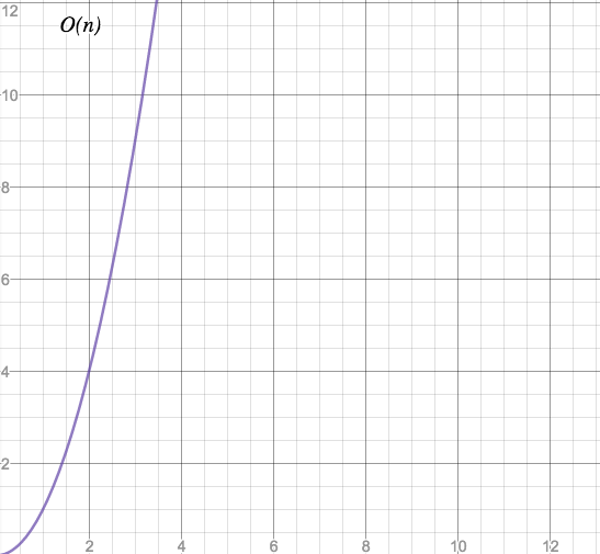
Plotted as a graph where the x axis is our input size n and the y axis are the time units needed to process n items, our term looks like this:

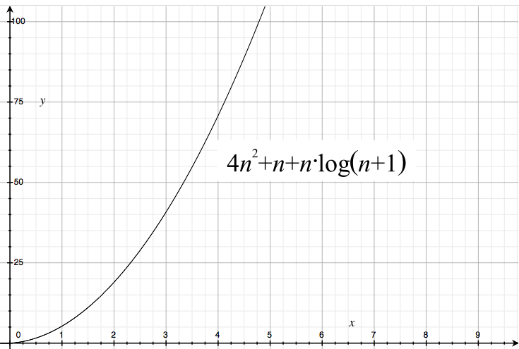
We can already see that with a raising number of items (x axis), processing time raises quickly - one item takes 5 time units, two items 20 units, three items 40 units, and so forth.

Can we leave some parts of the term away without changing this graph too much?

Obviously, we need to identify the part of the term that has the biggest influence on the shape of the graph. Let's divide the term into its components:

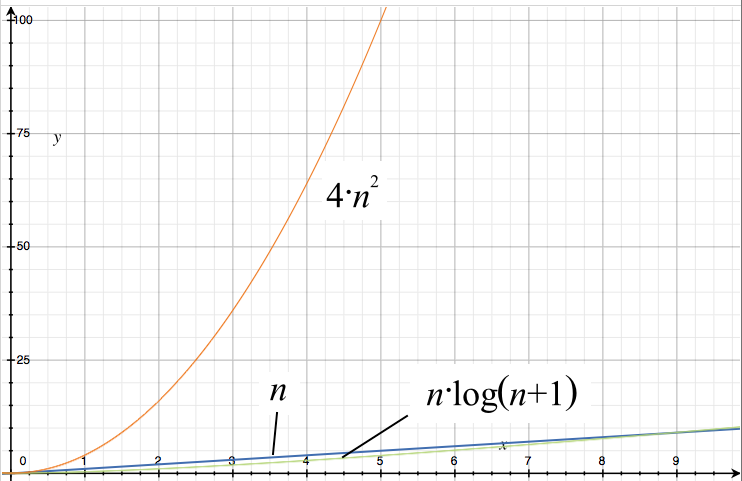
The orange graph corresponds to the term 4*n^2, the blue one to n, and the green one to n*log(n+1). It looks like wie can reduce our term to 4*n^2 without changing the characteristic shape of the graph.

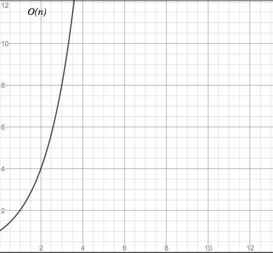
Can we simplify more? Let's take away the constant factor “4”:

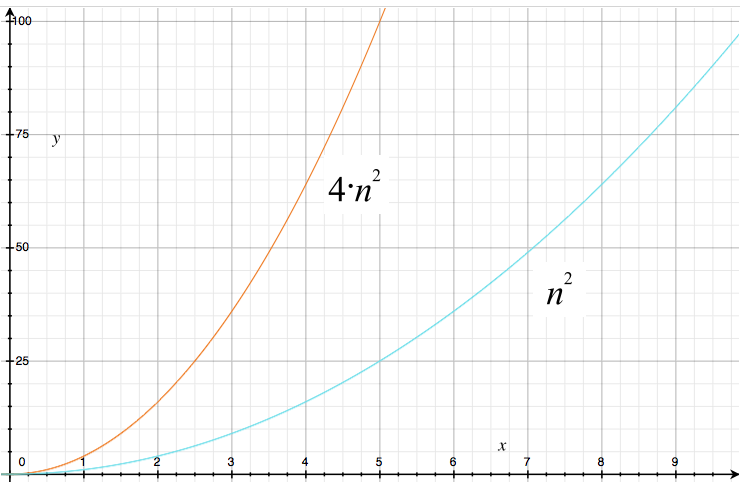
The new curve (cyan) looks less steep than the original one. However, their shapes are very similar, and so is their behavior when the input size is growing. The curves first grow slowly, then faster, and finally they shoot towards infinity, as we can see in this image where both axes have been scaled by a factor of 100:

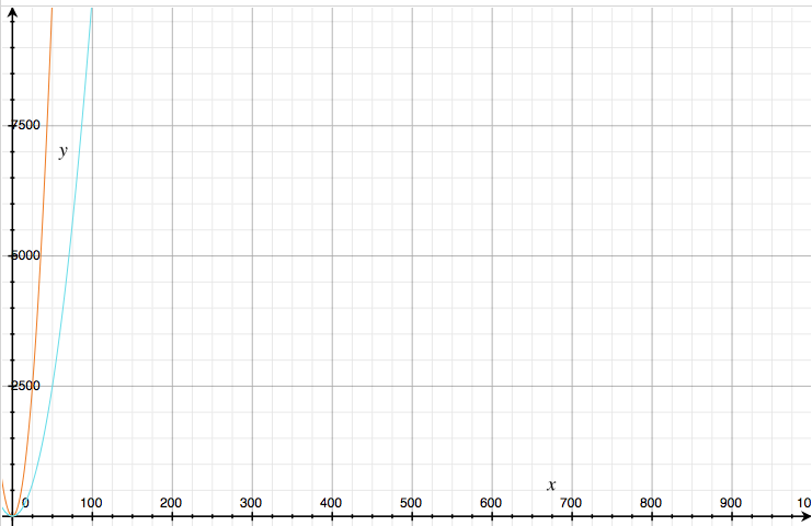
So for estimating purposes, we can even leave out the constant factor. Our term has now shrunken to a simple n^2, and the shape still resembles the original curve.

Now we safely can say that our imaginary code needs roughly n^2 units of time to process n items. Much easier than the bulky term we started with!

Takeaway: From all the terms that describe the time a function needs for processing an input of specific size, we only need that part of the term that has the largest effect.

The Big-O notation

The simplified term n^2 stands for a whole class of terms, so let's give it a name.

A function that needs roughly n^2 units of time to process n input items has a time complexity of O(n^2).

In general, we can say that -

A Big-O function is a mathematical term that gives a rough estimation of how the speed of an algorithm changes with the size of the input data.

Now we have a means to categorize time complexity into classes. Here are the most common classes:

O(1) - constant time

Characteristic: Instant delivery.

The code always needs the same time, no matter how large the input set is.

Graph:

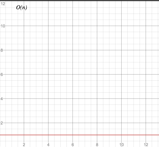
Example: Accessing a single element in an array of n items is an O(1) operation.

O(log(n)) - logarithmic time

Characteristic: The more data, the better.

The time the code needs to process n elements raises much slower than n for large values of n.

Graph:

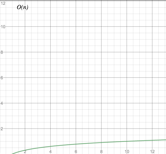
Examples: Inserting or retrieving elements into or from a balanced binary tree. Performing a binary search on a sorted array.

O(n) - linear time

Characteristic: One at a time.

Time needed for processing n element grows linearly with n.

Graph:

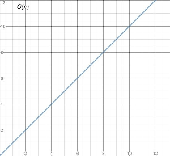
Examples: Iterating over an array, reading a file from start to end,

O(n*log(n)) - linearithmic time

Whoa, who invents these names?! “Linearithmic” is an artificial blend of “linear” and “logarithmic”, similar to “Brangelina”. (Bonus question: Which came first?)

Characteristic: Almost, but not quite, linear.

Somewhere between O(n) and O(n^2). Looks slightly like a flat O(n^2) curve for small values of n, and turns into an almost linear curve for large values of n.

Graph:

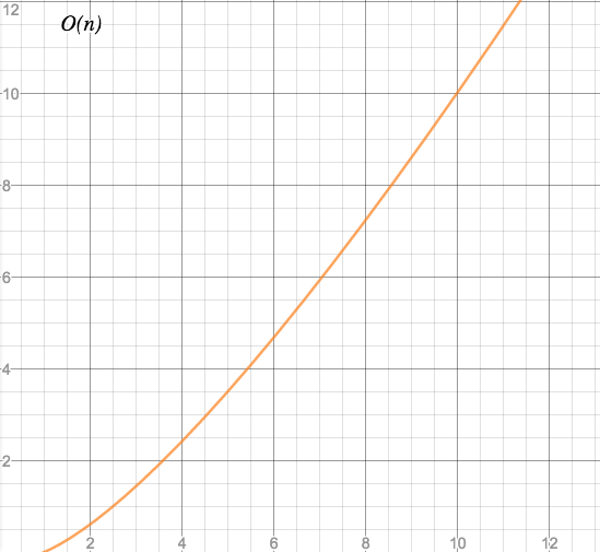
Examples: Heapsort, merge sort, binary tree sort

O(n^m) - polynomial time

For a given m > 0.

Characteristic: “Easy, fast, and practical.” (But quickly getting slow.)

Processing time raises fast. For O(n^2), when input size doubles, execution time quadruples. For O(n^3), double input size means eightfold execution time. And so on.

Here is where the danger zone comes into sight. With increasing n, polynomial algorithms quickly become slow.

Still, Cobham's thesis considers polynomial problems as “easy, fast, and practical”. Which means there are worse time complexities on the horizon.

Our O(n^2) problem from above belongs this class. This specific case is also called “quadratic time”.

(Nitpicking: O(n) would also belong to the polynomial class, since n is the same as n^1 and therefore a polynomial term, but due to its special “linear” nature it defines a separate class.)

Graph:

Examples: Bubble sort (O(n^2)). Any nested loops: Two nested loops - O(n^2). Three nested loops - O(n^3) and so on.

O(2^n) - exponential time

Characteristic: Here be dragons.

Even for moderate values of n, processing time goes through the roof.

Graph:

Example: The famous Traveling Salesman Problem: Find the shortest route between n towns. There are different approaches to this problem, but none of them belongs to a complexity class below O(2^n).

Comparison

The different characteristics of these time complexity classes become apparent when we put all those functions into one figure:

(Note: “n” has been replaced by “x” in the following two figures, as the graph tool did not let me specify n instead of x in the formulas.)

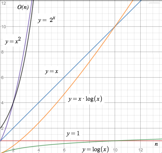
Here we can see immediately how the computation time diverges between the different complexity classes.

The graphs of O(n^2) and O(2^n) look as if they move very close together; however, after scaling the y axis to [0-200], the difference becomes obvious.

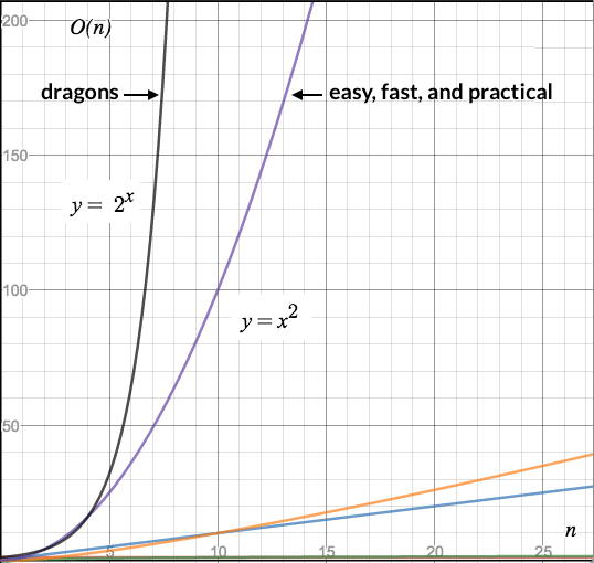
I know what you are thinking: This looks just like the difference between the graphs of 4*n^2 and n^2 - I said that difference is irrelevant, and now with this almost identical graph I claim that the difference matters. Let me show the point.

Imagine we can speed up the O(n^2) algorithm by any constant factor m. The curve will get flatter and flatter with increasing values of m, as the following graph demonstrates.

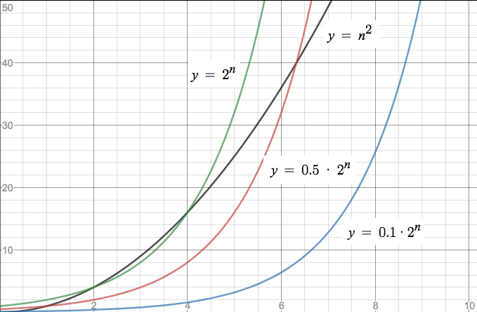
The black line is the polynomial function n^2, the green line is the exponential function 2^n, and the red and blue ones are the exponential function multiplied by a factor of 0.5 and 0.1, respectively. The blue one looks much better than the polynomial curve. So can O(2^n) beat O(n^2) just by a linear speedup?

Yes and no. For small values of n this can indeed happen. However, remember that we want to find out how an algorithm behaves when the input gets larger and larger. So let's scale the graph to see how the curves behave for larger values of n:

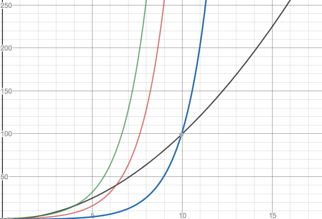
Now even the “flat” blue curve crosses the black one! Try this at home with even tinier values - at some n, the exponential curve will cross the polynomial one and increase much faster than the polynomial curve ever can. The difference between polynomial and exponential is indeed fundamental. (This applies to any pair of complexity classes.)

Improving O(n)

Looking at some of the curves, one question arises: Can we improve a given code, mabye even shift it into a faster Big-O class?

Change the algorithm

Let me give you a very practical answer here:

If the algorithm you strive to improve is one of the well-known, well-researched algorithms, the chances to find an equivalent, yet unknown, algorithm in a better complexity class is roughly zero. If you do find one, you are the hero of the day.

If, on the other hand, you are looking at some piece of lousy home-grown code, hacked together quickly while recovering from a severe hangover, then your chances aren't that bad. Read on…

Pre-process the input data

In some cases, the time complexity can be improved by re-arranging the input data.

For example, if you need to search through a list repeatedly (and much more often than adding something to this list), it will pay off to sort this list before searching it. A sorted list can be searched in O(log(n)) time using a binary search. Sure, sorting needs time, but you would have to do it only once to speed up those, say, thousands of searches that occur afterwards.

A good sort algorithm takes O(n*log(n)) time but reduces the time for each of the subsequent searches from O(n) to O(log(n)). Or for all n searches from O(n^2) to O(n*log(n). Big win!

Change your data structure

Sometimes it pays off inspecting the way your input data is stored.

Example: Inserting a new value into a sorted linear list takes O(n) time, as all values after the newly inserted one have to be shifted by one cell.

(Note we are talking about average times here, in individual cases, these operations may take less time. E.g., if the new value is inserted at the end, there is nothing to shift.)

(And another note: You may point out that finding the right place for inserting takes also some time, and for a sorted linear list, this would be O(log(n)) when using binary search, so the exact formula would be O(n + log(n)); however, as we have seen in the section “Simplifying the term”, using the most influential term of the sum is sufficient. In this scenario, this term is n.)

If you insert new data very frequently, better turn this list into a balanced tree. Then inserting a new value only takes O(log(n)) time. (Remember, log(n) is about the height of a balanced binary tree.)

Trade in time for space

So far we discussed only time complexity, but the same problem (and the same complexity classes) exists for memory consumption as well. Why not trading in one for the other?

One technique to exploit this is called “memoization”.

The idea behind memoization is: If a function is repeatedly called for the same input that is hard to calculate, store the results in memory and reuse them instead of re-calculating the same over and over.

As an example, calculating the factorial of n requires n multiplications.

func fac(n int) int {
	if n == 0 {
		return 1
	} else {
		return n * fac(n-1)
	}
}

This wrapper function stores all results in a map, and if a given n has already been calculated, it returns the result from the map; otherwise it calls fac(n).

func facm(n int, m map[int]int) int {
	r, ok := m[n]
	if ok {
		return r
	} else {
		r = fac(n)
		m[n] = r
		return r
	}
}

(Playground code here.)

The memoized function starts with the same time complexity as the original faculty function. Over time, however, most calls to facm() only require one map access (and although the Go Language Specification makes no performance guarantees for map access, we can safely assume that it is better than O(2^n)).package big-o

Use approximations and heuristics

Optimization problems like the Travelling Salesman problem (let's call it “TSP” henceforth) may have just one exact solution, but multiple near-optimal solutions. Algorithms that find near-optimal solutions by approximation and heuristics usually belong to a better O(n) class than the exact algorithm.

As an example, in the nearest neighbour algorithm, the salesperson, when arriving in one of the cities that are on the agenda, simply chooses the nearest unvisited city as the next destination, until all cities are visited.

On average, the path resulting from this strategy is 25% longer than the result from an exact algorithm, while the Nearest Neighbor algorithm only needs O(n^2) time.

Other strategies include ant colony optimization, simulated annealing, and genetic algorithms.

Can parallel execution achieve a better complexity class?

Given that goroutines can execute in parallel (provided that more than one (physical) CPU core is available), a question comes to mind: Can a parallel version of an algorithm belong to a better complexity class than the original serial algorithm?

For example, could the TSP be solved in O(n^2) rather than in O(2^n) (while still using an exact algorithm and no heuristics)?

Unfortunately, no.

To explain this, we do not even dive into complexity theory. We just need to look at the hardware: Two CPU cores can provide double speed at most, three can provide triple speed, and so forth. Adding CPU cores therefore speeds up execution only by a constant factor, and as we have seen in the introduction, constant factors are not relevant when talking about time complexity classes.

Conclusion

Time complexity and Big-O classes might seem tedious stuff but are enormously useful for predicting how code behaves when the input size grows. There is an abyss of theory behind all this, but this basic set of complexity classes should suffice for everyday use.

Links (as far as not already appearing in the text)

Wikipedia: Time complexity

Wikipedia: Big O notation

All but the first three graphs were created with the wonderful Desmos online graph calculator.

Happy coding!

Errata

2017-07-02: Fix the example in “Change your data structure”.